Project No. One: Microsoft Word
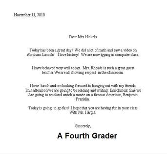 |
Letter to Challenger Staff Member
|
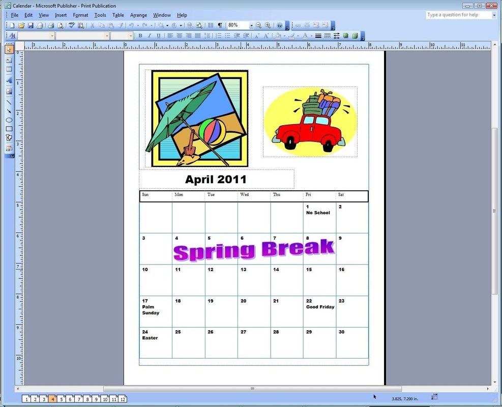
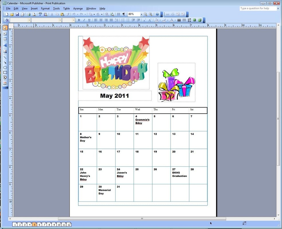
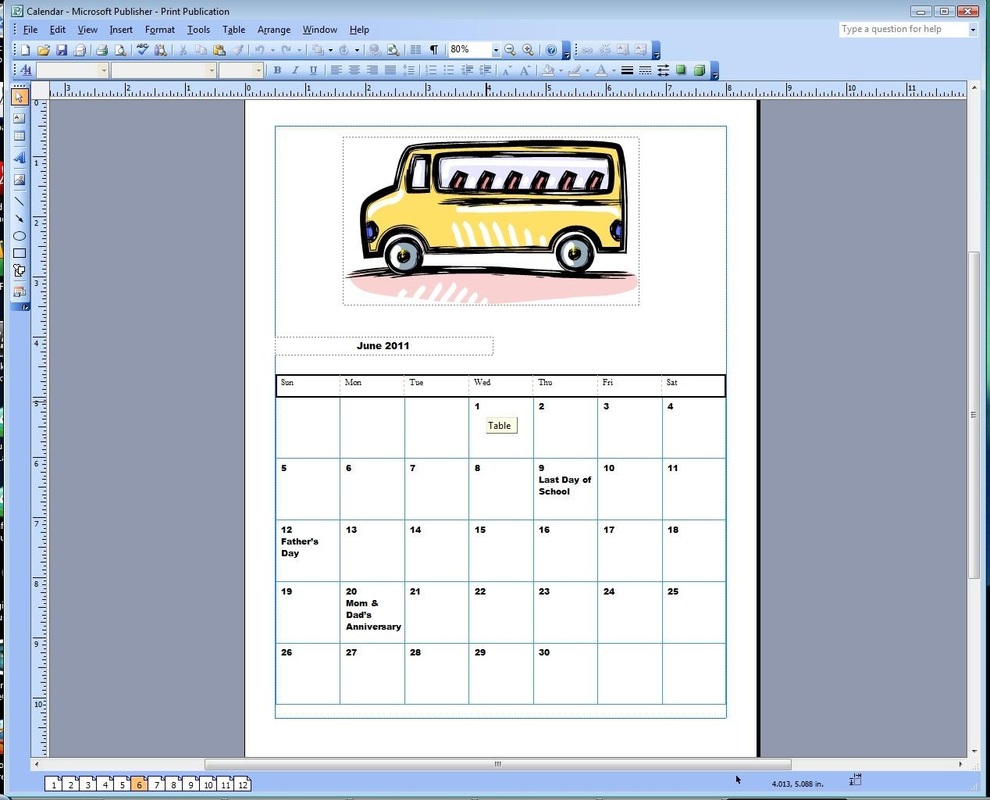
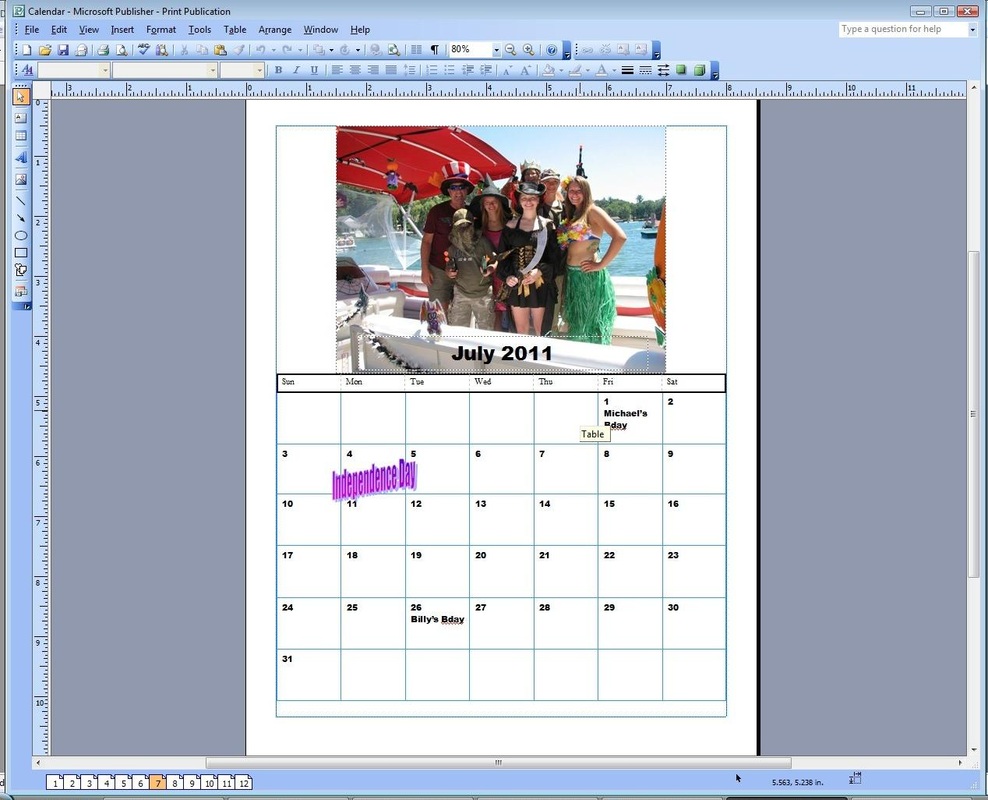
Project No. Two: Microsoft Publisher
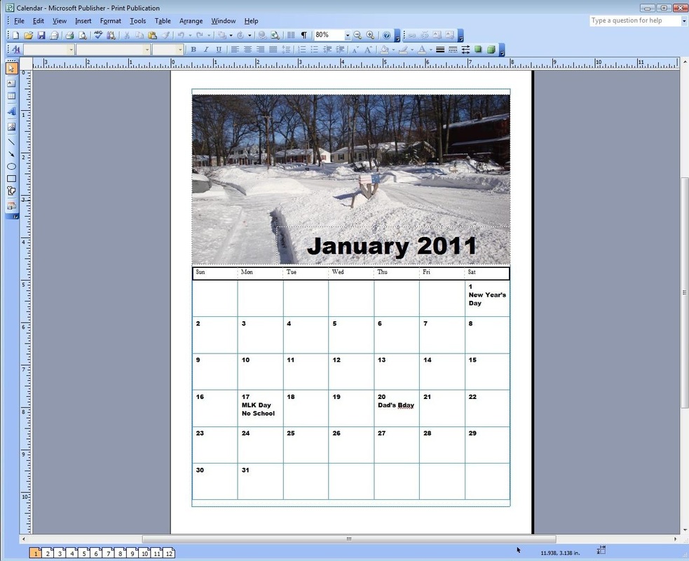
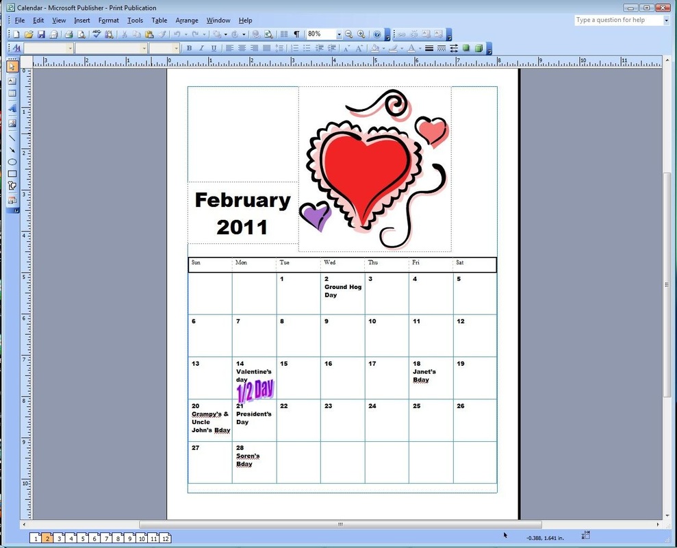
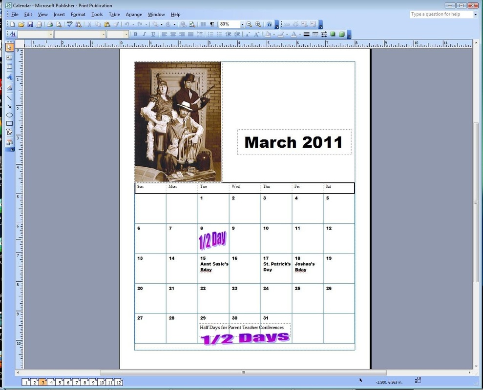
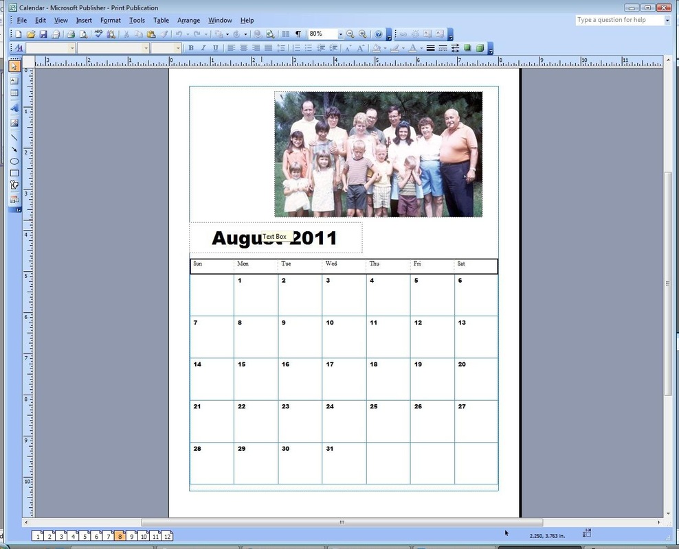
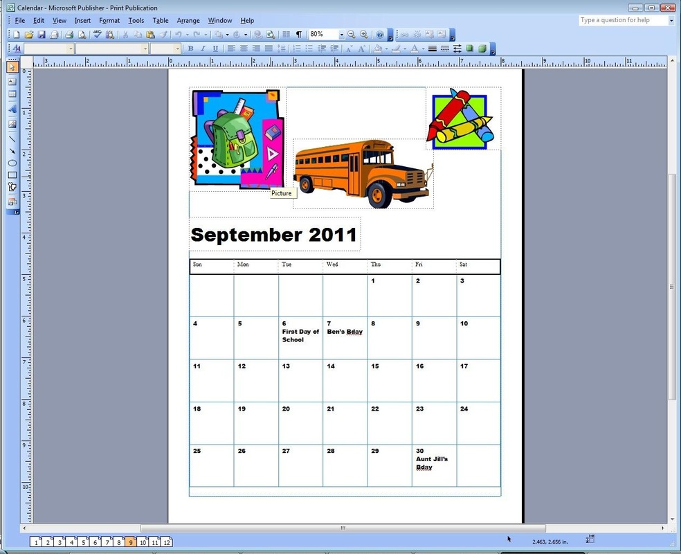
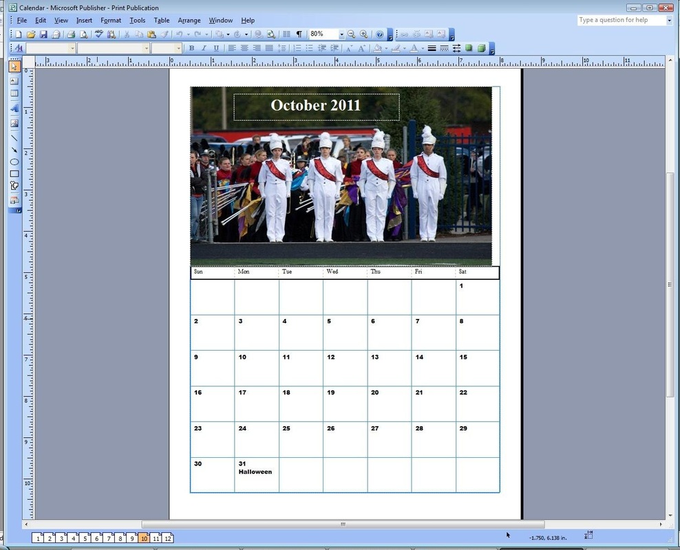
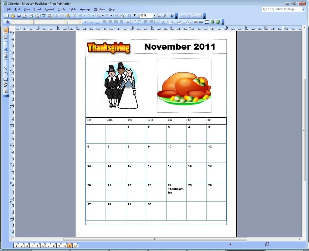
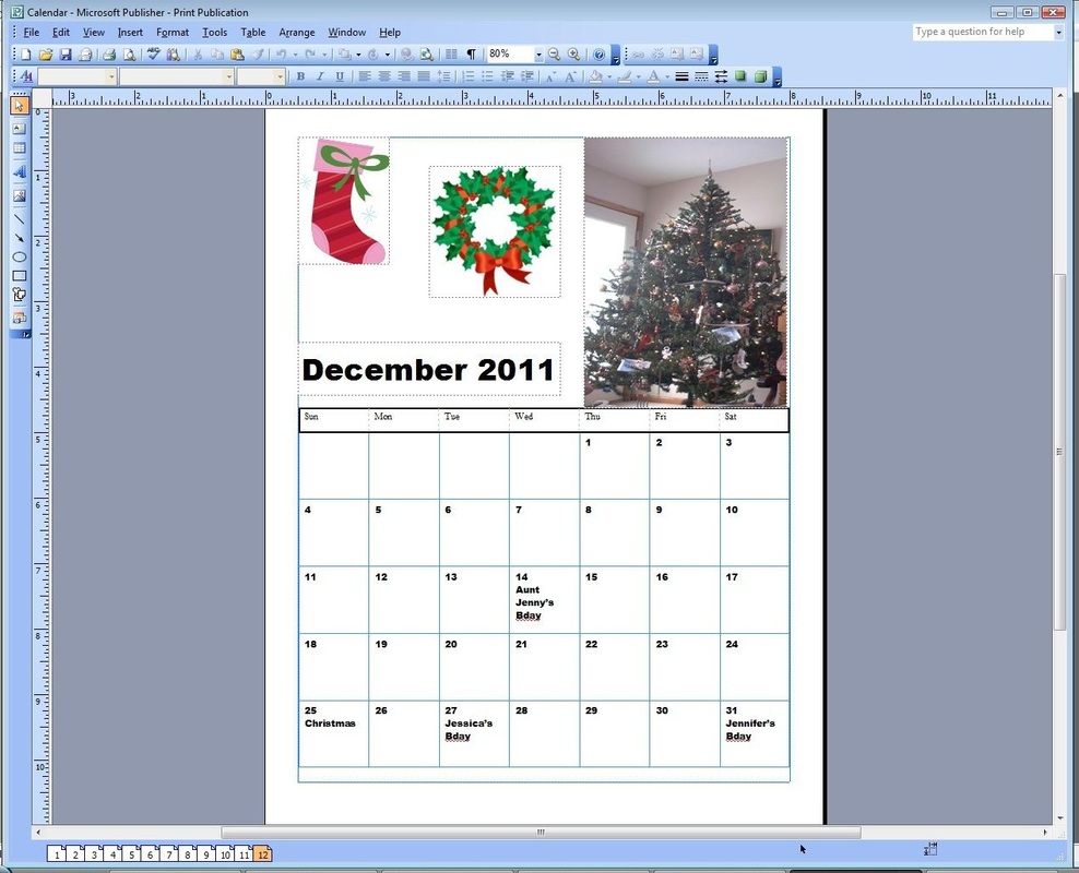
A Calendar to Take Home
|
            |
Project No. Three: Microsoft Excel Spreadsheet
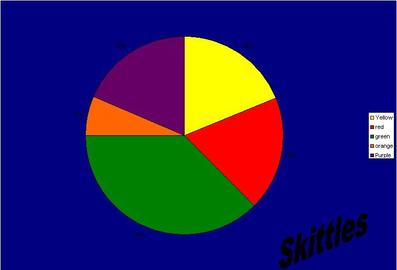 Skittles Analysis
1. Open Microsoft
Excel
2. In cell A1, type Skittles Analysis. Press Enter. 3. In cell A2 type: Colors. Press Enter. 4. Click in cell B2 and type: Number of Skittles. Press Enter. 5. In column A starting with cell A4 type in the colors surveyed. Press Enter after each color name to move to the next cell. 6. Change the font colors of each Skittle listed to match it. Do this by clicking on the word then the drop down arrow next to the font color icon. 7. In column B, enter the number of Skittles surveyed. 8. Skip 1 entire row and in column A under the last color, type Total. 9. In column B, next to Total, cell B , use the AUTOSUM button to total the number of Skittles. Press Enter. 10. Spell Check you work. 11. Before you make your chart, save your work – File- Save As – Drop Down Menu – Student on EKELEM – Teacher’s Folder – Press Enter – Student’s Folder – Press Enter – File Name – Skittles Analysis – Initials – Grade and Letter – Click Save. |
12. Highlight the cells that contain only the color
names and the number of Skittles. DO
NOT highlight the Title or the Total.
13. On the Insert Menu, select Chart, then select Pie or bar graph, as a chart type. Press and hold to view sample. This is to ensure that every student has highlighted the correct information. Click Next. 14. Click Next again. 15. Click in the Titles tab, enter Skittles Analysis in the Chart Title box. 16. Click on the Legend Tab, in the show legend option click where you want the legend to appear on your chart. 17. Click on the Data Labels tab and select the Category Value. Click Next. 18. Click on the As New Sheet Radio button so that the chart will appear on a page by itself and not on the spreadsheet. Click finish. 19. Zoom to 75%. 20. Notice that the colors are the same on your chart. Click on one section and change the colors to match your Skittles color. 21. Click the fill color can drop down arrow and select the correct color. Repeat with each section so you have different colors for each Skittle. Background 22. Zoom to 50% 23. Click on the white area or background around the pie so handles appear on the background. 24. Click Fill Color Can drop down arrow. Click Fill Effect. Choose the Gradient Tab. Choose Preset Colors. Select a color combination you like. Click OK. Play around and try different effects. Name 25. Click on the Word Art on the Drawing Toolbar 26. Select a Word Art you would like. Click OK. 27. Type in your name. Click OK. 28. Reposition your name on an empty place on your chart and reduce the size. |
Project No. Four: Microsoft Powerpoint
A Personal Interview with Me
|
|
